Multi-Year Energy Asset Planning Platform

Energy infrastructure planning requires answering three critical questions: what to build, when to build it, and how to operate it as technology costs, demand, and renewable availability evolve over decades. Traditional approaches rely on manually defined scenarios—planners compare predefined portfolios one-by-one, risking missed opportunities in the vast combinatorial space of asset mixes and timing. This platform replaces scenario enumeration with direct optimization: a mixed-integer linear programming (MILP) framework that automatically discovers cost-optimal asset schedules over 30-year horizons, explicitly tracking commissioning, operation, and retirement. Developed as an MSE project evolution from VT1's LP-based scenario comparison, VT2 validates lifecycle-aware optimization on a 5-bus network with 11 generation assets, 4 storage units, and 3× demand growth—solved in under 10 minutes on commodity hardware.

Technical Approach

The platform centers on MILP optimization for multi-year asset scheduling with lifecycle-aware constraints.

MILP Optimization Framework

Binary Decision Variables form the core of the lifecycle-aware optimization. Two binary variables per asset per year enable explicit modeling of commissioning and operational status. The optimizer chooses when to commission each asset (build decisions), while operational status is automatically determined by constraint as the sum of all unexpired builds within the asset's lifespan.

Lifecycle Management couples operational status with asset retirement through lifetime-aware constraints. Each asset has a defined lifespan (4-30 years in the candidate pool), with operational status determined by unexpired commissioning decisions. An "at-most-one-build-per-lifetime" constraint prevents overlapping installations within the same lifetime window. This formulation explicitly models asset aging, replacement cycles, and capacity evolution as load grows from baseline to 3× demand by year 30 (3% annual growth years 1-15, 5% thereafter).

Annualized Cost Modeling enables fair economic comparison across assets with different lifespans. The Capital Recovery Factor (CRF) converts upfront capital costs into equivalent annual payments:

CRF = [i(1+i)ⁿ] / [(1+i)ⁿ - 1]

Where i is the discount rate (5-10%) and n is asset lifetime in years. This annualization distributes capital costs evenly across operational years, avoiding end-of-horizon distortions and enabling direct comparison of short-lived storage (10-12 years) against long-lived thermal generators (25-30 years).

Implementation example:

def compute_crf(lifetime, discount_rate):
    i, n = discount_rate, lifetime
    return (i * (1 + i)**n) / ((1 + i)**n - 1)

annual_cost = capex * compute_crf(lifetime, discount_rate)

Vectorized Constraint Formulation achieved 50-100× computational speedup versus VT1's loop-based LP implementation. Constraints for 10,000+ optimization variables (binary commissioning decisions, continuous dispatch variables, storage state-of-charge tracking) are built using NumPy array operations and passed to IBM CPLEX solver. Representative week aggregation (one week per season) reduces temporal resolution while preserving seasonal dispatch patterns, enabling multi-decade planning horizons with solve times under 10 minutes on M4 MacBook Pro.

Results & Validation

Multi-Year Asset Deployment

The 30-year planning horizon automatically discovered optimal commissioning schedules for all candidate assets (11 generators + 4 storage units) on a 5-bus network. Demand grows 3× from baseline through compound annual rates (3% years 1-15, 5% years 16-30), imposing continuous pressure to expand capacity and replace aging assets.

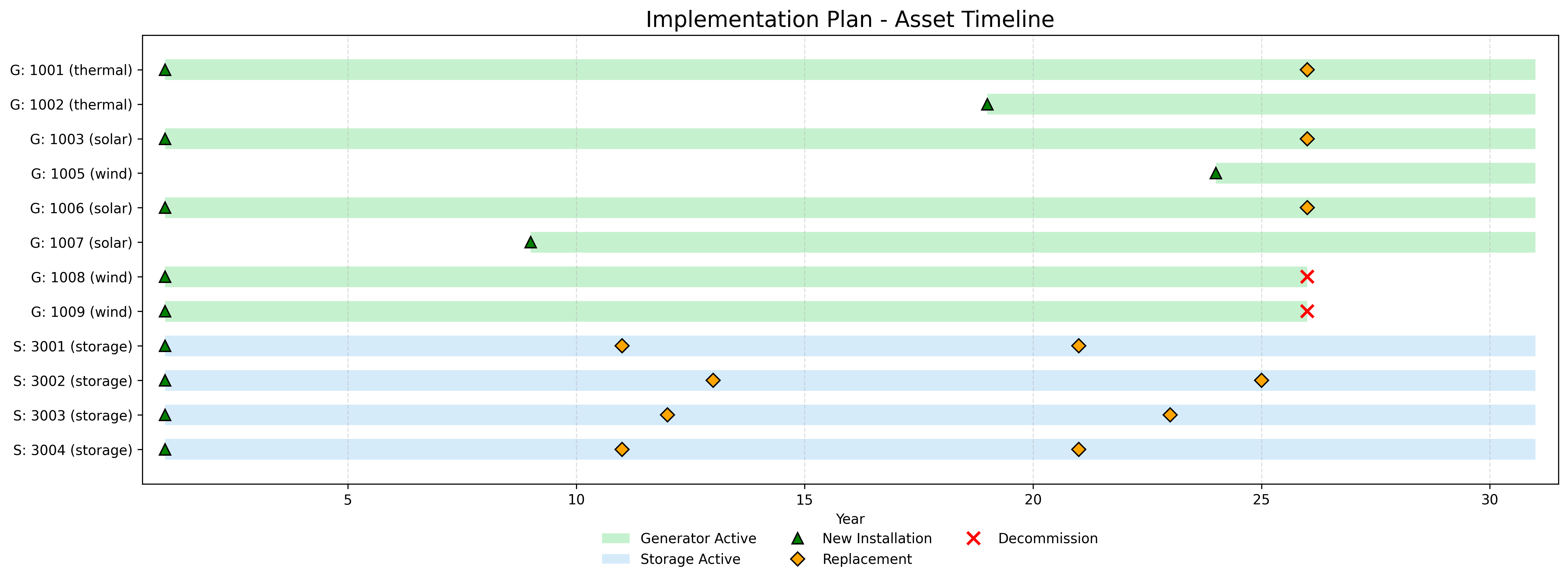30-year infrastructure roadmap: Storage deployed immediately (year 1), renewables expanded progressively, thermal capacity deferred until year 19 as demand triples. Horizontal bars span asset operational lifetimes (4-30 years), with replacements scheduled at end-of-life.

Analysis: The optimizer exhibits strong preference for early deployment of zero-fuel-cost renewable assets (solar, wind) despite shorter lifespans (25 years) compared to thermal generators (30 years). All 4 storage units commission in year 1, demonstrating economic viability beyond operational flexibility—storage enables renewable integration and peak-shaving value that outweighs 10-12 year replacement cycles. Thermal Generator 2 defers to year 19, reflecting fuel cost penalty in the objective function. By year 30, existing assets operate at maximum utilization before new commissioning—evidence of solver efficiency and load pressure driving infrastructure to capacity limits.

Generation Mix Evolution

Seasonal dispatch patterns reveal how the system adapts to load growth and renewable penetration over three decades. Winter and summer representative weeks demonstrate contrasting operational regimes.

Year 1 vs. Year 30 Comparison:

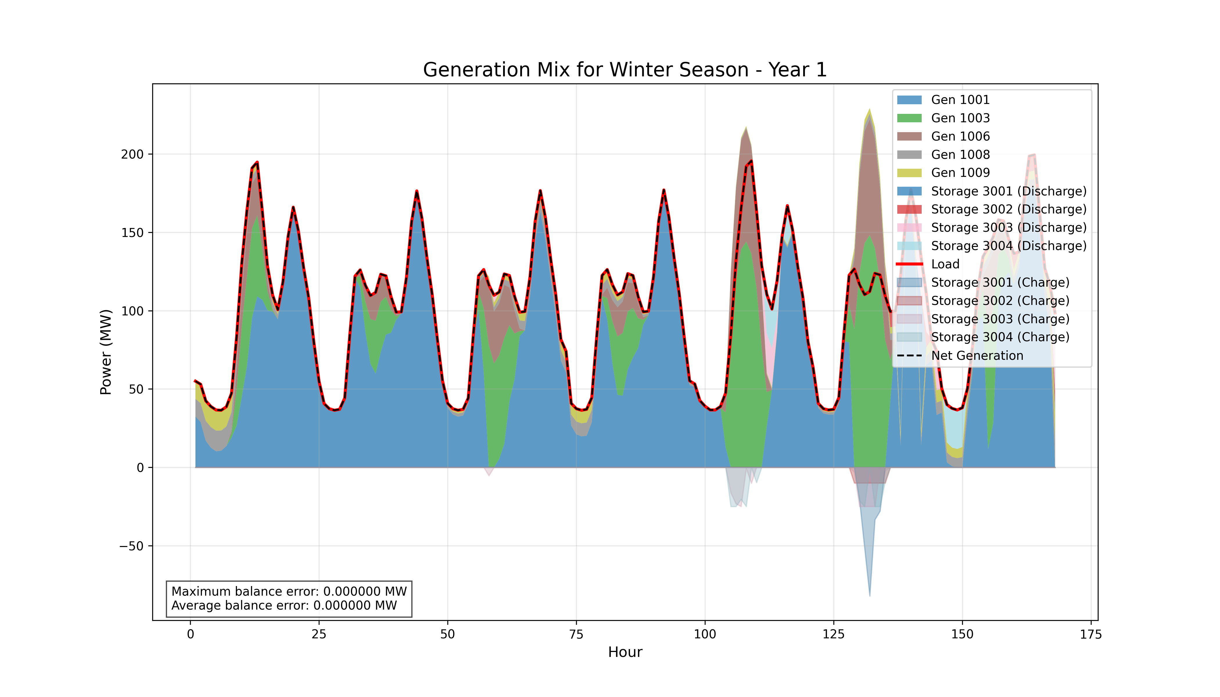Winter week dispatch, Year 1: Thermal-dominated operation with nascent storage support. Renewables provide supplemental capacity during peak daylight hours.

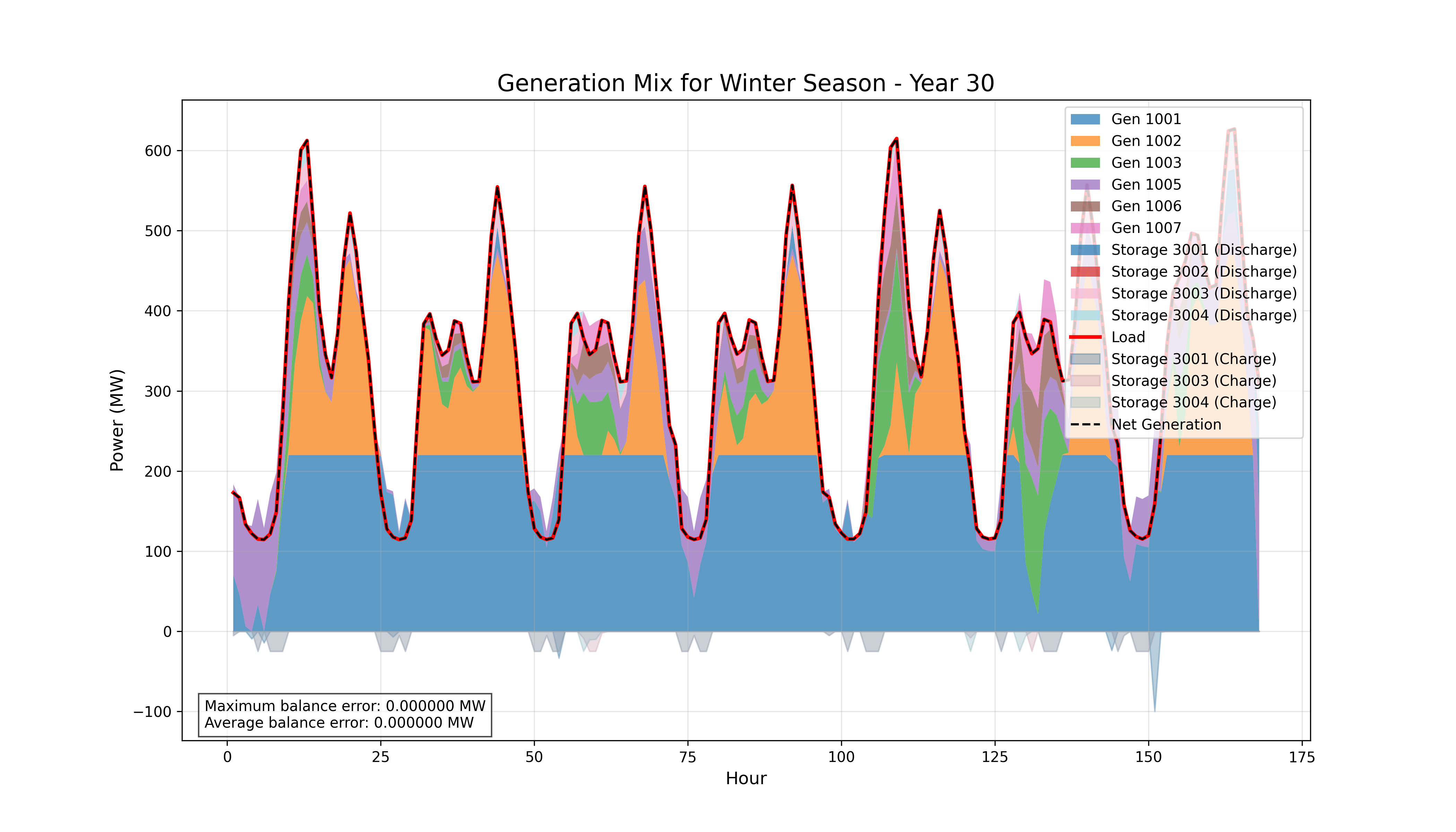Winter week dispatch, Year 30: Thermal remains primary baseload as demand triples, with expanded storage role managing ramps and renewable variability. Storage capacity increased through replacements (10-12 year cycles).

Winter analysis: Thermal generation dominates both years due to lower solar irradiance and higher heating loads. By year 30, storage exhibits pronounced charge/discharge cycling to smooth renewable ramps and defer thermal peaking. Load growth (3× baseline) drives thermal capacity to maximum sustained output, with renewables filling mid-day valleys.

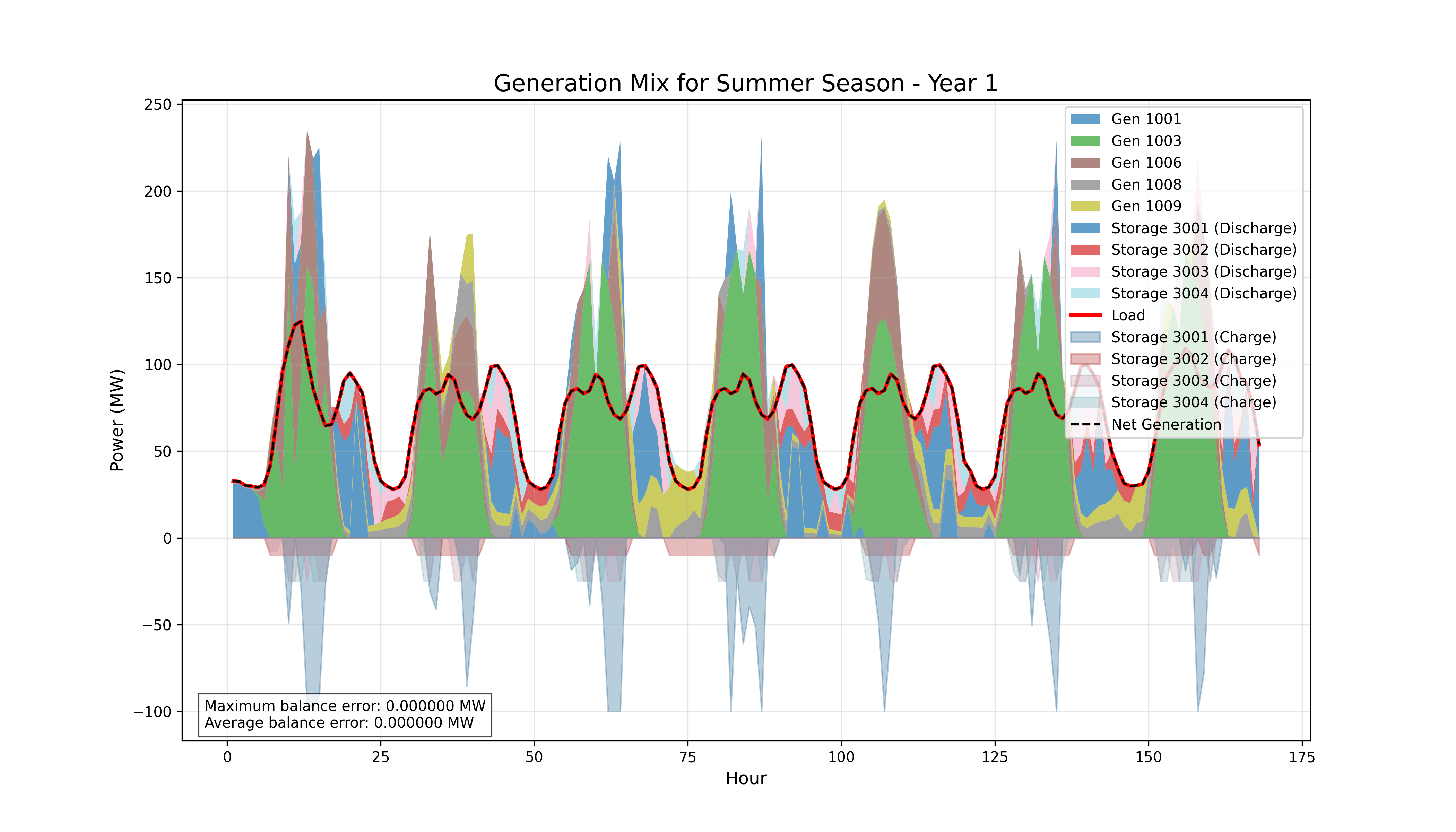Summer week dispatch, Year 1: Balanced mix with solar contributing during mid-day peaks. Limited storage cycling due to lower renewable penetration.

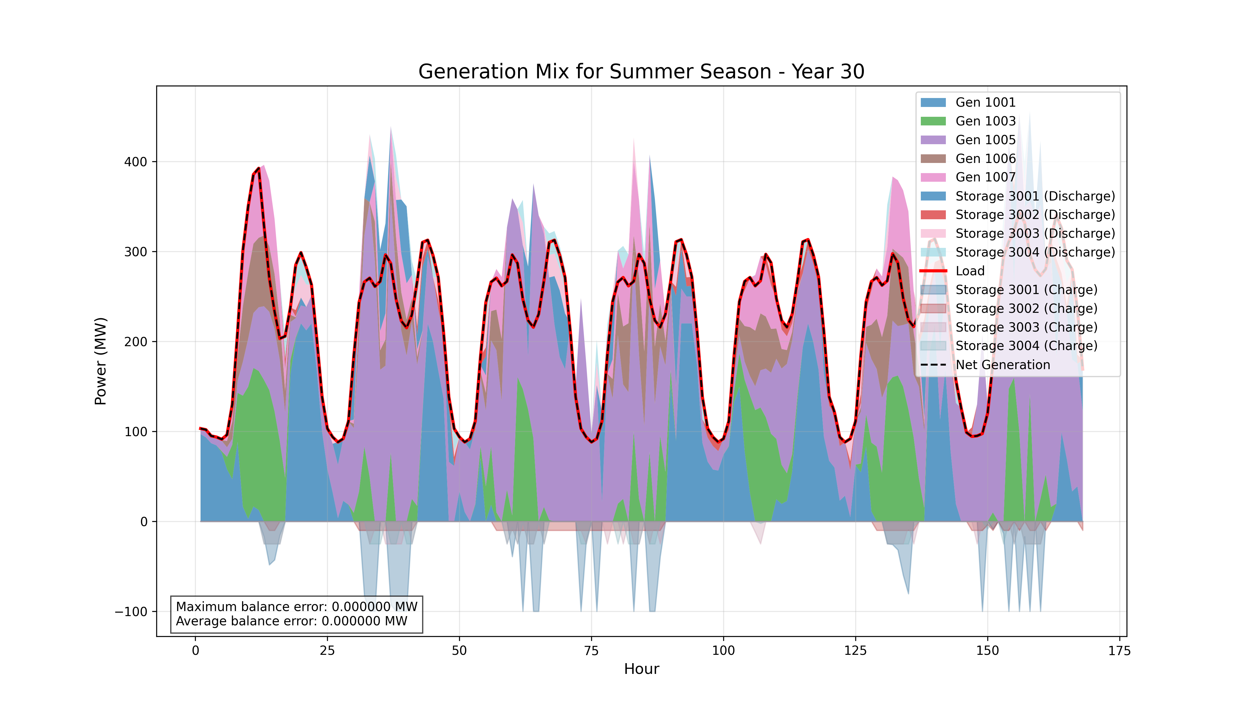Summer week dispatch, Year 30: Solar dominance during daylight hours with deep storage cycling. "Duck curve" mitigation evident—storage charges during midday surplus, discharges during evening ramp. Thermal reduced to residual/peaking role.

Summer analysis: By year 30, solar generation dominates mid-day operations, creating pronounced surplus that charges storage to full capacity. Evening demand ramps trigger deep discharge cycles, mitigating the "duck curve" challenge. Thermal generators transition from baseload to peaking/residual role, operating at minimum stable levels during high-solar periods. The optimizer automatically discovered this seasonal differentiation through cost minimization—zero-fuel renewables displace thermal during high-irradiance months.

Outcomes

The platform delivers four key capabilities for energy infrastructure planning:

Unified Planning Tool: Co-optimizes investment timing and operational dispatch over 30-year horizons in a single MILP formulation. Binary variables for commissioning decisions interact with continuous dispatch variables through lifetime-aware constraints, eliminating the artificial separation between strategic planning and operational scheduling that characterizes traditional scenario-based approaches.

Automatic Asset Selection: Eliminates manual scenario enumeration—the optimizer discovers cost-optimal portfolios from the full candidate pool (11 generators + 4 storage in this validation) without analyst-defined cases. Traditional methods require defining dozens of "what-if" scenarios; MILP collapses this combinatorial space into direct optimization, surfacing solutions potentially missed by intuition-driven scenario selection.

Lifecycle Awareness: Explicit retirement and replacement scheduling aligned with technical lifespans (4-30 years) and load evolution. The annualized cost formulation (CRF) distributes capital expenditure across operational years, enabling fair comparison between short-lived storage (10-12 years) and long-lived thermal generators (30 years) while avoiding end-of-horizon distortions common in NPV-only approaches.

Technical Validation

• Planning horizon: 30 years with compound load growth (3% → 5% annual, final 3× demand)
• Network scale: 5-bus grid, 11 generation assets (thermal/solar/wind), 4 storage units
• Optimization variables: 10,000+ (binary commissioning + continuous dispatch + storage SoC)
• Solve time: <10 minutes (M4 MacBook Pro, IBM CPLEX)
• Computational speedup: 50-100× versus VT1's loop-based LP formulation

Key Insights

Economic preference for renewables: Zero-fuel-cost solar and wind deploy early despite shorter lifespans (25 years) versus thermal (30 years). CAPEX disadvantage outweighed by operational savings—demonstrating the value of annualized cost modeling that captures lifecycle economics rather than upfront capital bias.

Storage as infrastructure: All 4 storage units commissioned year 1, demonstrating strategic value beyond operational flexibility. Storage enables renewable integration (absorbing mid-day solar surplus) and peak-shaving (deferring thermal expansion), with economic return justifying 10-12 year replacement cycles throughout the horizon.

Scalability vs. tractability: Representative-week aggregation (1 week per season) enables multi-decade horizons with <10 min solve times but limits rare-event modeling (extreme weather, grid stress). Future work must balance temporal detail with computational tractability for large networks (100+ buses).

Limitations & Future Work

The current implementation demonstrates proof-of-concept lifecycle optimization but requires several extensions for production deployment:

Representative weeks aggregate temporal detail, capturing seasonal patterns but missing rare stress events (extreme weather, multi-day renewable lulls, grid contingencies). Full 8760-hour resolution becomes computationally intractable beyond 5-10 year horizons—future work must explore temporal clustering methods that preserve extremes while maintaining tractability.

Deterministic optimization assumes perfect foresight of load growth and renewable availability. Real planning requires stochastic MILP formulations that optimize under uncertainty—incorporating forecast error distributions, demand variability, and technology cost projections.

Binary annual investments assume assets commission at year-start, ignoring gradual capacity additions common in utility-scale projects (phased wind farm build-out, modular storage expansion). Relaxing to partial-year commissioning or continuous capacity variables may better represent incremental investments while increasing problem complexity.

Future directions: Stochastic MILP for renewable/demand uncertainty propagation; ramp constraints and maintenance scheduling (currently ignored); scalability testing on 100+ bus networks; validation on real utility planning cases with historical load/renewable data.

The project demonstrates that energy infrastructure decisions benefit from simultaneous lifecycle and operational modeling—enabling planners to evaluate portfolios based on long-term economics and short-term operational constraints rather than optimizing each dimension independently.